Conic Sections
Table of Contents
- 1. Equations
- 2. Discriminant
- 3. Conjugate Axes
- 4. Principal Axes
- 5. Similarity
- 6. Projective Geometry
- 7. Circle
- 8. Ellipse
- 9. Hyperbola
- 10. Parabola
- 11. Quadric
- 12. Reference
- A section of a bicone.
1. Equations
1.1. General Form
\[ Ax^2+Bxy+Cy^2+Dx+Ey+F=0. \]
1.2. Matrix Form
\[ \mathbf{x}^{\mathrm{T}}\mathbf{A}\mathbf{x}=0 \] where \[ \mathbf{x}=\begin{bmatrix}x\\ y \\1\end{bmatrix}\quad \mathbf{A}=\begin{bmatrix}A&B/2&D/2\\B/2&C&E/2\\D/2&E/2&F\end{bmatrix} \]
1.3. Vector Form
- Extraordinary Conics: The Most Difficult Math Problem I Ever Solved - YouTube
- A set with size five of points and lines can define a conic section.
- \[ \mathbf{x}=\mathbf{a}\sin(\theta)+\mathbf{b}\cos(\theta)+\mathbf{c} \] or \[ \mathbf{x}=\mathbf{a}\sinh(\theta)\pm\mathbf{b}\cosh(\theta)+\mathbf{c} \] for any non-colinear vectors \(\mathbf{a}, \mathbf{b}\).
- Area \[ A=\pi|\mathbf{a}\times\mathbf{b}| \]
- \(c^2\) Invariant \[ c^2=\mathbf{a}^2+\mathbf{b}^2 \]
Interiority Test
\begin{equation*} |(\mathbf{p}-\mathbf{c})\times \mathbf{a}|^2+|(\mathbf{p}-\mathbf{c})\times\mathbf{b}|^2< |\mathbf{a}\times\mathbf{b}|^2 \end{equation*}- Tangency Test
where \(\mathbf{p}\) is the point of tangency and \(\mathbf{r}\) is the direction in which the tangent line is.
1.4. Points Form
Given 9 points(18 degrees of freedom) within the affine space \(v_1, v_2, \dots, v_9\) with 9 collinearity conditions(removes 8 degrees of freedom since the last condition is dependent to the previous), by the Pappus's hexagon theorem:
\begin{equation*} |v_7, v_8, v_9| = \frac{|v_1, v_5, v_4||v_3, v_4, v_6||v_2, v_6, v_5||v_1, v_2, v_3| - |v_1, v_5, v_2||v_3, v_4, v_1||v_2, v_6, v_3||v_4, v_5, v_6|}{|v_1, v_5, v_2-v_4||v_3, v_4, v_1-v_6||v_2, v_6, v_3-v_5|} = 0. \end{equation*}Let any of the 6 points, say \(v_6\) be the variable:
\begin{equation*} v = \begin{bmatrix} x \\ y \\ 1 \end{bmatrix} \end{equation*}Yielding the equation of a conic section that contains h \(v_1, v_2, \dots, v_5\):
\begin{equation*} |v_1, v_5, v_4||v_3, v_4, v||v_2, v, v_5||v_1, v_2, v_3| - |v_1, v_5, v_2||v_3, v_4, v_1||v_2, v, v_3||v_4, v_5, v| = 0. \end{equation*}- This holds due to the Pascal's theorem.
- Braikenridge-Maclaurin theorem guerantees the existence of the conic containing five points.
2. Discriminant
- \( B^2 - 4AC \)
It is \(-4\Delta\) where \(\Delta\) being the minor \(m_{3,3}\) of the quadratic form.
For the non-degenerate conic
- If \(-4\Delta < 0\), it is an ellipse
- If \(-4\Delta = 0\), it is a parabola
- If \(-4\Delta > 0\), it is a hyperbola
This method checks, for a given \( y \), how many \( x \) satisfy the conic equation: 0 for ellipse, 1 for parabola, 2 for parabola.
Alternatively, \(\Delta\) can be used
- If \(\Delta > 0\), it is an ellipse
- If \(\Delta = 0\), it is a parabola
- If \(\Delta < 0\), it is a hyperbola
Since the matrix is symmetric, only stretchings in orthogonal direction are possible. It checks for the eigenvalues, and one of the eigenvalues equals to zero for parabola negative for hyperbola.
3. Conjugate Axes
- Each chord parallel to one diameter is bisected by the other diameter.
- For an ellipse, the conjugate diameter is parallel to the tangent line to the ellipse at an endpoint of the one diameter.
3.1. Intuition
For an ellipsoid centered at the origin, the ellipsoid corresponds to a quadratic form
\begin{equation*} \mathbf{x}^\top \mathbf{A} \mathbf{x} = 1 \end{equation*}where \( \mathbf{x} \) is the coordinate vector.
The vectors that represent conjugate axes \( \{ v_i \} \) are the set of vectors that satisfy:
\begin{equation*} \mathbf{v}_i^{\top} \mathbf{A}\mathbf{v}_j = \delta_{ij}. \end{equation*}4. Principal Axes
- where eigenvalues of \(A_{33}\) forms the principal axes.
- Principal axis theorem states that they are orthogonal to each other.
5. Similarity
- By similar, affine transformation is meant.
- the Holy Trinity of curves - YouTube
- Every ellipse is similar to the unit circle.
- Every hyperbola is similar to the unit hyperbola.
- Every parabola is similar to the unit parabola.
- They are not similar to each other in the real plane.
- However, ellipses and parabolas are similar to each other in the complex plane.
6. Projective Geometry
6.1. Homogenization
- \[ Ax^2+2Bxy+Cy^2+2Dxz+2Eyz+Fz^2=0 \]
6.2. Bicone
7. Circle
7.1. Equation of Circle
- Standard form
- \( (x-x_0)^2+(y-y_0)^2=r^2 \)
- General form
- \( ax^2+by^2+cx+dy+e=0 \) where \(a=b\).
- Circle with diameter \(\rm\overline{AB}\)
- \( (x-a_x)(x-b_x)+(y-a_y)(y-b_y)=0 \)
- In vector notation, \( (\mathbf{x}-\mathbf{a})\cdot(\mathbf{x}-\mathbf{b})=0 \) which describes all the points such that vector from \( \rm A \)and vector from \( \rm B \)are perpendicular.
- Vector form
- \( (\mathbf{x}-\mathbf{x}_0)\cdot(\mathbf{x}-\mathbf{x}_0)=r^2 \)
7.2. Circle from Three Points
- This task is usually a chore – not anymore! - YouTube
- A circle is completely defined by any three non-colinear points \(\rm A,B, C\).
- From the equation of circle with diameter \(\rm\overline{AB}\), \(f(x,y)=0\) and the equation of line that goes through \(\rm A,B\), \(g(x,y)=0\), one can find a real number \(\alpha\) such that \(f(x,y)=\alpha g(x,y)\) contains all three points.
7.3. Circles of Apollonius
- Points with a fixed ratio of distances from two points form a circle.
8. Ellipse
8.1. Equation
8.1.1. Standard Equation
- \[ \frac{x^2}{a^2} + \frac{x^2}{b^2} = 1 \]
8.1.2. General From
- \[
Ax^2 + Bxy + Cy^2 + Dx + Ey + F = 0
\]
- with \(B^2 - 4AC < 0\).
8.1.2.1. Conversion to the Canonical Form
- \[ a, b = \frac{-\sqrt{2 \big(A E^2 + C D^2 - B D E + (B^2 - 4 A C) F\big)\big((A + C) \pm \sqrt{(A - C)^2 + B^2}\big)}}{B^2 - 4 A C} \]
- \[ x_\circ = \frac{2CD - BE}{B^2 - 4AC} \]
- \[ y_\circ = \frac{2AE - BD}{B^2 - 4AC} \]
- \[
\theta = \frac{1}{2} \operatorname{atan2}(-B,\, C-A)
\]
- with atan2 function.
8.1.3. Canonical Form
- \[
\frac{((x-x_\circ)\cos\theta + (y-y_\circ)\sin\theta)^2}{a^2} + \frac{(-(x-x_\circ)\sin\theta + (y-y_\circ)\cos\theta)^2}{b^2} = 1
\]
- by the Euclidean transformation of the coordinates of the canonical equation.
8.1.3.1. Conversion to the General Form
- \(A = a^2\sin^2\theta + b^2\cos^2\theta\)
- \(B = 2(b^2 - a^2)\sin\theta\cos\theta\)
- \(C = a^2\cos^2\theta + b^2\sin^2\theta\)
- \(D = -2Ax_\circ - By_\circ\)
- \(E = -Bx_\circ - 2Cy_\circ\)
- \(F = Ax_\circ^2 + Bx_\circ y_\circ + Cy_\circ^2 - a^2b^2\)
8.1.4. Parametric
- \[
\mathbf{x} = \mathbf{f}_0 + \mathbf{f}_1\cos t + \mathbf{f}_2\sin t
\]
- The unit circle \((\cos t, \sin t)\) after the affine transformation \(\mathbf{x}\mapsto \mathbf{f}_0 + A\mathbf{x}\), where \(A\) is a square matrix with \(\mathbf{f}_1, \mathbf{f}_2\) as the column vectors.
- \(\mathbf{f}_1, \mathbf{f}_2\) are the conjugate diameters.
8.1.4.1. Vertices
- \(\mathbf{x}(t_0 + m\pi/2)\), where: \[ \cot(2 t_0) = \frac{\mathbf{f}_1^2 - \mathbf{f}_2^2}{2\mathbf{f}_1\cdot \mathbf{f}_2}. \]
- This is obtained from the relation: \[ \frac{d\mathbf{x} }{dt}\cdot (\mathbf{x} - \mathbf{f}_0)\Big|_{t=t_0} = 0. \]
8.1.4.2. Area
- \[ A = \pi|\det(\mathbf{f}_1, \mathbf{f}_2)| \]
8.1.4.3. Intercepts
- For the ellipse
\(\mathbf{x} = \mathbf{a}\cos\theta + \mathbf{b}\sin\theta\)
- \[ x_{\rm intercept} = \frac{\vec{a}\times \vec{b}}{\sqrt{a_y^2+b_y^2}}\cdot \hat{k} \]
- \[ y_{\rm intercept} = \frac{\vec{b}\times \vec{a}}{\sqrt{a_x^2+b_x^2}}\cdot \hat{k} \]
8.1.4.4. Conversion to the Implicit Form
- \[ \det(\mathbf{x}-\mathbf{f}_0, \mathbf{f}_2)^2 + \det(\mathbf{f}_1,\mathbf{x}-\mathbf{f}_0)^2 - \det(\mathbf{f}_1, \mathbf{f}_2)^2 = 0 \]
- This is obtained by solving \(\sin t, \cos t\) with Cramer's rule and applying \(\cos^2 t + \sin^2 t - 1 = 0\).
- It is an equation in \(x\) and \(y\).
8.1.5. Polar Form
8.1.5.1. Angles
- The tangential angles are identical when measured form the either foci.
8.1.5.2. Relative to the Center
- \[
r = \frac{ab}{\sqrt{(b\cos\theta)^2 + (a\sin\theta)^2}} = \frac{b}{\sqrt{1-(e\cos\theta)^2}}\text{ or } \frac{a}{\sqrt{1-(e\sin\theta)^2}}
\]
- if \(a>b\) the former, if \(b>a\) the latter.
- This can be obtained by plugging \(x = r\cos\theta, y = r\cos\theta\) in the Cartesian form of the equation.
- \(\theta\) is called the true anomaly.
8.1.5.3. Relative to the Focus
- \[ r = \frac{\ell}{1\pm e\cos\theta} \] assuming \(a>b\).
- This is obtained by applying to the triangle subtended from the two foci by a point on the perimeter.
- The angle \(\theta\) is called the true anomaly of the point.
- \(\ell = a(1-e^2)\) is the semi-latus rectum.
8.2. Parameters
8.2.1. Semi-Major Axis and Semi-Minor Axis
- 장축, 단축
- The length of the semi-major axis and semi-minor axis is commonly
denoted by \(a\) and \(b\).
- 장반경, 단반경
- \[ b = a^2 - c^2 = \sqrt{1-e^2}a \]
8.2.2. Focus
- \( F \)
- Focal Point
8.2.2.1. Focal Distance
- Linear Eccentricity
- The distance between the center and the focus, commonly denoted with \(c\).
8.2.3. Vertex
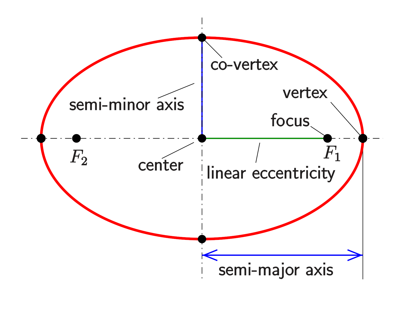
- The points on the principal axis.
8.2.4. Apocenter and Pericenter
- peri-, 'near'
- Sometimes, apapsis and periapsis
- The furthest and nearest point from one of the focus.
- I will denote the radius from the focus at apocenter and pericenter with \(r_{\rm ap}\) and \(r_{\rm per}\)
- \[ r_{\rm ap} = a+c = (1+e)a \]
- \[ r_{\rm per} = a -c = (1-e)a \]
- See apsis
- \[ \ell = (1+e)r_{\rm per} \]
- \[ a = \frac{1}{1-e}r_{\rm per} \]
8.2.5. Eccentricity
- The ratio of linear eccentricity, the length from the center to
one of the foci, with respect to the semi-major axis:
\[
e := \frac{c}{a} = \frac{\sqrt{a^2 - b^2}}{a} = \sqrt{1-\frac{b^2}{a^2}}
\]
- where \(a\) is the semi-major axis.
8.2.6. Semi-Latus Rectum
- Sometimes, Latus Rectum
- The length of the line through the foci perpendicular to the major axis.
- \[
\ell = \frac{b^2}{a} = (1-e^2)a
\]
- \(a\ell = b^2\)
- It can be seen as the relation between arithmetic, geometric, and harmonic mean
- \[
\frac{\ell}{1+e} = r_{\rm per}\quad
\frac{\ell}{1-e} = r_{\rm ap}
\]
- directly form the polar equation relative to the center
8.2.7. Circumference
- No elementary formula exists.
- The formula is given as follows1, 2:
- \[ \pi\sum_{n=0}^{\infty}\left( \frac{1\cdot 3\cdot 5\cdots (2n-3)}{2^{n}\cdot n!} \right)^2\frac{(a-b)^{2n}}{(a+b)^{2n-1}} \]
- Using the elliptic integral:
- \[ C = 4a E(e) \]
- where \(a\) is the semi-major axis, \(e\) is the eccentricity, and \(E\) is the complete elliptic integral of the second kind.3
8.2.8. Angular Parameters
Anomalies
8.2.8.1. True Anomaly
8.2.8.2. Eccentric Anomaly
8.2.8.3. Mean Anomaly
The angle that would have been made if the orbit was circular.
8.3. Relations
- For an ellipse parameterized by \((\cos\theta, a\sin\theta)\), at
every point:
- \[ r^2 = 1+e^2y^2. \]
- Apsis
- \[
a = \frac{r_{\rm ap} + r_{\rm per}}{2}
\]
- \[ c = \frac{r_{\rm ap} - r_{\rm per}}{2} \]
- \[ b = \sqrt{ r_{\rm ap}r_{\rm per} } \]
- \[ \ell = \left( \frac{r_{\rm ap}^{-1} + r_{\rm per}^{-1}}{2}\right)^{-1} \]
- \[ e = \frac{r_{\rm ap} - r_{\rm per}}{r_{\rm ap} + r_{\rm per}} \]
- \[
a = \frac{r_{\rm ap} + r_{\rm per}}{2}
\]
- Tangential Angle
- \[
\sin\phi = \frac{b}{\sqrt{r(2a-r)}}
\]
- where \(\phi\) is the angle of the tangent line with respect to one of the segments from the foci, and \(r\) is the length of one of the segments.
- This can be obtained from the :
- \[ \begin{align*} (2c)^2 &= r^2 + s^2 - 2rs\cos(\pi - 2\phi)\\ \implies (2c)^2 &= (r+s)^2 - 4rs\sin^{\cdot 2}\phi \\ \implies \sin\phi &= \sqrt{\frac{(2a)^2 - (2c)^2}{4rs}} \end{align*} \]
- The same form can also be derived independently from the angular momentum conservation and energy conservation.
- Proof of Kepler's Elliptical Orbit Law
- \[
\sin\phi = \frac{b}{\sqrt{r(2a-r)}}
\]
9. Hyperbola
9.1. Unit Hyperbola
- \[ x^2 - y^2 = 1 \]
9.2. Special Hyperbolae
- \[ y = \frac{1}{x} \iff 1 = \frac{1}{xy} \iff xy = 1 \]
9.3. Scaling a Hyperbola
- Scaling in one of the axes: \[ y = \frac{1}{(kx)} \iff ky = \frac{1}{x} \] is equivalent to scaling in both axes by the square root of the factor: \[ \sqrt{k}y = \frac{1}{\sqrt{k} x}. \]
9.4. Hyperbolic Rotation
- It can be thought of squishing in the direction of one of the asymptote, and stretching it the direction of the other asymptote by the same factor, .
- When The wedges under the hyperbola gets hyperbolically rotated, the total area is preserved, which is similar to the rotation of a circle.
- It can be represented by a symmetric matrix with determinant of one.
9.5. Hyperbolic Functions
10. Parabola
10.1. Properties
- The points \( (a, a^2), (b, b^2), (0,ab) \) are colinear.
- What's Behind the Parabola? (#SoME3) - YouTube
11. Quadric
- Quadric Surface, Quadric Hypersurface
- Generalization of the conic sections.
11.1. Definition
- The affine # Algebraic Variety in the form of \[ \mathbf{x}^{\rm T}\mathbf{Q}\mathbf{x} + \mathbf{P}\mathbf{x} + R = 0. \]
12. Reference
- https://en.wikipedia.org/wiki/Conic_section#Conic_parameters
- https://en.wikipedia.org/wiki/Conjugate_diameters
- https://en.wikipedia.org/wiki/Principal_axis_theorem
- https://en.wikipedia.org/wiki/Ellipse
- Eccentric anomaly - Wikipedia
- https://en.wikipedia.org/wiki/Eccentricity_(mathematics)
- Quadric - Wikipedia